- 1 Introduction to Data Science
- 2 Reading in data locally and from the web
- 2.1 Overview
- 2.2 Chapter learning objectives
- 2.3 Absolute and relative file paths
- 2.4 Reading tabular data from a plain text file into R
- 2.5 Reading data from an Microsoft Excel file
- 2.6 Reading data from a database
- 2.7 Writing data from R to a
.csvfile - 2.8 Scraping data off the web using R
- 2.9 Additional readings/resources
- 3 Cleaning and wrangling data
- 3.1 Overview
- 3.2 Chapter learning objectives
- 3.3 Vectors and Data frames
- 3.4 Tidy Data
- 3.5 Combining functions using the pipe operator,
%>%: - 3.6 Iterating over data with
group_by+summarize - 3.7 Additional reading on the
dplyrfunctions - 3.8 Using
purrr’smap*functions to iterate - 3.9 Additional readings/resources
- 4 Effective data visualization
- 5 Introduction to Data Science
Chapter 5 Introduction to Data Science
5.1 Loading a spreadsheet-like dataset
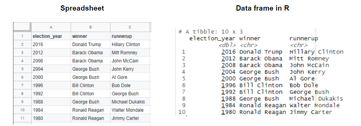
Often, the first thing we need to do in data analysis is to load a dataset into R. When we bring spreadsheet-like (think Microsoft Excel tables) data, generally shaped like a rectangle, into R it is represented as what we call a data frame object. It is very similar to a spreadsheet where the rows are the collected observations and the columns are the variables.
The first kind of data we will learn how to load into R (as a data frame) is the
spreadsheet-like comma-separated values format (.csv for short).
These files have names ending in .csv, and can be opened open and saved from common spreadsheet programs like Microsoft Excel and Google Sheets.
For example, a .csv file named state_property_vote.csv is included with the code for this book.
This file— originally from Data USA—has US state-level property, income, population and voting data from 2015 and 2016.
If we were to open this data in a plain text editor, we would see each row on its own line, and each entry in the table separated by a comma:
state,med_income,med_prop_val,population,mean_commute_minutes,party
AK,64222,197300,733375,10.46830207,Republican
AL,36924,94800,4830620,25.30990746,Republican
AR,35833,83300,2958208,22.40108933,Republican
AZ,44748,128700,6641928,20.58786,Republican
CA,53075,252100,38421464,23.38085172,Democrat
CO,48098,198900,5278906,19.50792188,Democrat
CT,69228,246450,3593222,24.349675,Democrat
DC,70848,475800,647484,28.2534,Democrat
DE,54976,228500,926454,24.45553333,Democrat
To load this data into R, and then to do anything else with it afterwards, we will need to use something called a function.
A function is a special word in R that takes in instructions (we call these arguments) and does something. The function we will
use to read a .csv file into R is called read_csv.
In its most basic use-case, read_csv expects that the data file:
- has column names (or headers),
- uses a comma (
,) to separate the columns, and - does not have row names.
Below you’ll see the code used to load the data into R using the read_csv function. But there is one extra step we need to do first. Since read_csv is not included in the base installation of R,
to be able to use it we have to load it from somewhere else: a collection of useful functions known as a library. The read_csv function in particular
is in the tidyverse library (more on this later), which we load using the library function.
Next, we call the read_csv function and pass it a single argument: the name of the file, "state_property_vote.csv". We have to put quotes around filenames and other letters and words that we
use in our code to distinguish it from the special words that make up R programming language. This is the only argument we need to provide for this file, because our file satifies everthing else
the read_csv function expects in the default use-case (which we just discussed). Later in the course, we’ll learn more about how to deal with more complicated files where the default arguments are not
appropriate. For example, files that use spaces or tabs to separate the columns, or with no column names.
clicking the below button will make this book interactive and that could take some times to strat. Be patient…
us_data <- readr::read_csv("https://raw.githubusercontent.com/UBC-DSCI/introduction-to-datascience/master/state_property_vote.csv")## Parsed with column specification:
## cols(
## state = col_character(),
## med_income = col_double(),
## med_prop_val = col_double(),
## population = col_double(),
## mean_commute_minutes = col_double(),
## party = col_character()
## )## Parsed with column specification:
## cols(
## state = col_character(),
## med_income = col_double(),
## med_prop_val = col_double(),
## population = col_double(),
## mean_commute_minutes = col_double(),
## party = col_character()
## )## # A tibble: 52 x 6
## state med_income med_prop_val population mean_commute_minutes party
## <chr> <dbl> <dbl> <dbl> <dbl> <chr>
## 1 AK 64222 197300 733375 10.5 Republican
## 2 AL 36924 94800 4830620 25.3 Republican
## 3 AR 35833 83300 2958208 22.4 Republican
## 4 AZ 44748 128700 6641928 20.6 Republican
## 5 CA 53075 252100 38421464 23.4 Democrat
## 6 CO 48098 198900 5278906 19.5 Democrat
## 7 CT 69228 246450 3593222 24.3 Democrat
## 8 DC 70848 475800 647484 28.3 Democrat
## 9 DE 54976 228500 926454 24.5 Democrat
## 10 FL 43355 125600 19645772 24.8 Republican
## # … with 42 more rowsAbove you can also see something neat that Jupyter does to help us understand our code: it colours text depending on its meaning in R. For example, you’ll note that functions get bold green text, while letters and words surrounded by quotations like filenames get blue text.
In case you want to know more (optional): We use the
read_csvfunction from thetidyverseinstead of the base R functionread.csvbecause it’s faster and it creates a nicer variant of the base R data frame called a tibble. This has several benefits that we’ll discuss in further detail later in the course.