Chapter 2 Reading in data locally and from the web

2.4.1 Skipping rows when reading in data

Often times information about how data was collected, or other relevant information, is included at the top of the data file. This information is usually written in sentence and paragraph form, with no delimiter because it is not organized into columns. An example of this is shown below:

Data source: https://datausa.io/
Record of how data was collected: https://github.com/UBC-DSCI/introduction-to-datascience/blob/master/data/src/retrieve_data_usa.ipynb
Date collected: 2017-06-06
state,med_income,med_prop_val,population,mean_commute_minutes,party
AK,64222,197300,733375,10.46830207,Republican
AL,36924,94800,4830620,25.30990746,Republican
AR,35833,83300,2958208,22.40108933,Republican
AZ,44748,128700,6641928,20.58786,Republican
CA,53075,252100,38421464,23.38085172,Democrat
CO,48098,198900,5278906,19.50792188,Democrat
CT,69228,246450,3593222,24.349675,Democrat
DC,70848,475800,647484,28.2534,Democrat
DE,54976,228500,926454,24.45553333,Democrat

Using read_csv as we did previously does not allow us to correctly load the data into R. In the case of this file we end up only reading in one column of the data set:

us_data <- read_csv("data/state_property_vote_meta-data.csv")

## Parsed with column specification:
## cols(
##   `Data source: https://datausa.io/` = col_character()
## )

us_data

## # A tibble: 55 x 1
##    `Data source: https://datausa.io/`                                                                  
##    <chr>                                                                                               
##  1 Record of how data was collected: https://github.com/UBC-DSCI/introduction-to-datascience/blob/mast…
##  2 Date collected: 2017-06-06                                                                          
##  3 state                                                                                               
##  4 AK                                                                                                  
##  5 AL                                                                                                  
##  6 AR                                                                                                  
##  7 AZ                                                                                                  
##  8 CA                                                                                                  
##  9 CO                                                                                                  
## 10 CT                                                                                                  
## # … with 45 more rows

To successfully read data like this into R, the skip argument can be useful to tell R how many lines to skip before it should start reading in the data. In the example above, we would set this value to 3:

us_data <- read_csv("data/state_property_vote_meta-data.csv", skip = 3)

## Parsed with column specification:
## cols(
##   state = col_character(),
##   med_income = col_double(),
##   med_prop_val = col_double(),
##   population = col_double(),
##   mean_commute_minutes = col_double(),
##   party = col_character()
## )

us_data

## # A tibble: 52 x 6
##    state med_income med_prop_val population mean_commute_minutes party     
##    <chr>      <dbl>        <dbl>      <dbl>                <dbl> <chr>     
##  1 AK         64222       197300     733375                 10.5 Republican
##  2 AL         36924        94800    4830620                 25.3 Republican
##  3 AR         35833        83300    2958208                 22.4 Republican
##  4 AZ         44748       128700    6641928                 20.6 Republican
##  5 CA         53075       252100   38421464                 23.4 Democrat  
##  6 CO         48098       198900    5278906                 19.5 Democrat  
##  7 CT         69228       246450    3593222                 24.3 Democrat  
##  8 DC         70848       475800     647484                 28.3 Democrat  
##  9 DE         54976       228500     926454                 24.5 Democrat  
## 10 FL         43355       125600   19645772                 24.8 Republican
## # … with 42 more rows

2.4.2 read_delim as a more flexible method to get tabular data into R

When our tabular data comes in a different format, we can use the read_delim function instead. For example, a different version of this same dataset has no column names and uses tabs as the delimiter instead of commas.

Here is how the file would look in a plain text editor:

AK  64222   197300  733375  10.46830207 Republican
AL  36924   94800   4830620 25.30990746 Republican
AR  35833   83300   2958208 22.40108933 Republican
AZ  44748   128700  6641928 20.58786    Republican
CA  53075   252100  38421464    23.38085172 Democrat
CO  48098   198900  5278906 19.50792188 Democrat
CT  69228   246450  3593222 24.349675   Democrat
DC  70848   475800  647484  28.2534 Democrat
DE  54976   228500  926454  24.45553333 Democrat
FL  43355   125600  19645772    24.78055522 Republican

To get this into R using the read_delim() function, we specify the first argument as the path to the file (as done with read_csv), and then provide values to the delim argument (here a tab, which we represent by "\t") and the col_names argument (here we specify that there are no column names be assigning it the value of FALSE). Both read_csv() and read_delim() have a col_names argument and the default is TRUE.

us_data <- read_delim("data/state_property_vote.tsv",  delim = "\t", col_names = FALSE)

## Parsed with column specification:
## cols(
##   X1 = col_character(),
##   X2 = col_double(),
##   X3 = col_double(),
##   X4 = col_double(),
##   X5 = col_double(),
##   X6 = col_character()
## )

us_data

## # A tibble: 52 x 6
##    X1       X2     X3       X4    X5 X6        
##    <chr> <dbl>  <dbl>    <dbl> <dbl> <chr>     
##  1 AK    64222 197300   733375  10.5 Republican
##  2 AL    36924  94800  4830620  25.3 Republican
##  3 AR    35833  83300  2958208  22.4 Republican
##  4 AZ    44748 128700  6641928  20.6 Republican
##  5 CA    53075 252100 38421464  23.4 Democrat  
##  6 CO    48098 198900  5278906  19.5 Democrat  
##  7 CT    69228 246450  3593222  24.3 Democrat  
##  8 DC    70848 475800   647484  28.3 Democrat  
##  9 DE    54976 228500   926454  24.5 Democrat  
## 10 FL    43355 125600 19645772  24.8 Republican
## # … with 42 more rows

Data frames in R need to have column names, thus if you read data into R as a data frame without column names then R assigns column names for them. If you used the read_* functions to read the data into R, then R gives each column a name of X1, X2, …, XN, where N is the number of columns in the data set.

2.4.3 Reading tabular data directly from a URL

We can also use read_csv() or read_delim() (and related functions) to read in tabular data directly from a url that contains tabular data. In this case, we provide the url to read_csv() as the path to the file instead of a path to a local file on our computer. Similar to when we specify a path on our local computer, here we need to surround the url by quotes. All other arguments that we use are the same as when using these functions with a local file on our computer.

us_data <- read_csv("https://raw.githubusercontent.com/UBC-DSCI/introduction-to-datascience/master/state_property_vote.csv")

## Parsed with column specification:
## cols(
##   state = col_character(),
##   med_income = col_double(),
##   med_prop_val = col_double(),
##   population = col_double(),
##   mean_commute_minutes = col_double(),
##   party = col_character()
## )

us_data

## # A tibble: 52 x 6
##    state med_income med_prop_val population mean_commute_minutes party     
##    <chr>      <dbl>        <dbl>      <dbl>                <dbl> <chr>     
##  1 AK         64222       197300     733375                 10.5 Republican
##  2 AL         36924        94800    4830620                 25.3 Republican
##  3 AR         35833        83300    2958208                 22.4 Republican
##  4 AZ         44748       128700    6641928                 20.6 Republican
##  5 CA         53075       252100   38421464                 23.4 Democrat  
##  6 CO         48098       198900    5278906                 19.5 Democrat  
##  7 CT         69228       246450    3593222                 24.3 Democrat  
##  8 DC         70848       475800     647484                 28.3 Democrat  
##  9 DE         54976       228500     926454                 24.5 Democrat  
## 10 FL         43355       125600   19645772                 24.8 Republican
## # … with 42 more rows

2.4.4 Previewing a data file before reading it into R

In all the examples above, we gave you previews of the data file before we read it into R. This is essential so that you can see whether or not there are column names, what the delimiters are, and if there are lines you need to skip. You should do this yourself when trying to read in data files. In Jupyter, you preview data as a plain text file by clicking on the file’s name in the Jupyter home menu. We demonstrate this in the video below:

2.6.1 Reading data from a SQLite database

SQLite is probably the simplest relational database that one can use in combination with R. SQLite databases are self-contained and usually stored and accessed locally on one computer. Data is usually stored in a file with a .db extension. Similar to Excel files, these are not plain text files and cannot be read in a plain text editor.

The first thing you need to do to read data into R from a database is to connect to the database. We do that using the dbConnect function from the DBI (database interface) package. This does not read in the data, but simply tells R where the database is and opens up a communication channel.

library(DBI)
con_state_data <- dbConnect(RSQLite::SQLite(), "data/state_property_vote.db")

Often times relational databases have many tables, and their power comes from the useful ways they can be joined. Thus anytime you want to access data from a relational database you need to know the table names. You can get the names of all the tables in the database using the dbListTables function:

tables <- dbListTables(con_state_data)
tables

## [1] "state"

We only get one table name returned form calling dbListTables, and this tells us that there is only one table in this database. To reference a table in the database so we can do things like select columns and filter rows, we use the tbl function from the dbplyr package:

library(dbplyr)
state_db <- tbl(con_state_data, "state")
state_db

## # Source:   table<state> [?? x 6]
## # Database: sqlite 3.31.1
## #   [/Users/tiffany/Desktop/introduction-to-datascience/data/state_property_vote.db]
##    state med_income med_prop_val population mean_commute_minutes party     
##    <chr>      <dbl>        <dbl>      <dbl>                <dbl> <chr>     
##  1 AK         64222       197300     733375                 10.5 Republican
##  2 AL         36924        94800    4830620                 25.3 Republican
##  3 AR         35833        83300    2958208                 22.4 Republican
##  4 AZ         44748       128700    6641928                 20.6 Republican
##  5 CA         53075       252100   38421464                 23.4 Democrat  
##  6 CO         48098       198900    5278906                 19.5 Democrat  
##  7 CT         69228       246450    3593222                 24.3 Democrat  
##  8 DC         70848       475800     647484                 28.3 Democrat  
##  9 DE         54976       228500     926454                 24.5 Democrat  
## 10 FL         43355       125600   19645772                 24.8 Republican
## # … with more rows

Although it looks like we just got a data frame from the database, we didn’t! It’s a reference, showing us data that is still in the SQLite database (note the first two lines of the output). It does this because databases are often more efficient at selecting, filtering and joining large datasets than R. And typically, the database will not even be stored on your computer, but rather a more powerful machine somewhere on the web. So R is lazy and waits to bring this data into memory until you explicitly tell it to do so using the collect function from the dbplyr library.

Here we will filter for only states that voted for the Republican candidate in the 2016 Presidential election, and then use collect to finally bring this data into R as a data frame.

republican_db <- filter(state_db, party == "Republican")
republican_db

## # Source:   lazy query [?? x 6]
## # Database: sqlite 3.31.1
## #   [/Users/tiffany/Desktop/introduction-to-datascience/data/state_property_vote.db]
##    state med_income med_prop_val population mean_commute_minutes party     
##    <chr>      <dbl>        <dbl>      <dbl>                <dbl> <chr>     
##  1 AK        64222        197300     733375                 10.5 Republican
##  2 AL        36924         94800    4830620                 25.3 Republican
##  3 AR        35833         83300    2958208                 22.4 Republican
##  4 AZ        44748        128700    6641928                 20.6 Republican
##  5 FL        43355        125600   19645772                 24.8 Republican
##  6 GA        37865        101700   10006693                 24.5 Republican
##  7 IA        49448        102700    3093526                 18.4 Republican
##  8 ID        43080.       143900    1616547                 19.9 Republican
##  9 IN        47194        111800    6568645                 23.5 Republican
## 10 KS        46875         85200    2892987                 16.7 Republican
## # … with more rows

republican_data <- collect(republican_db)
republican_data

## # A tibble: 31 x 6
##    state med_income med_prop_val population mean_commute_minutes party     
##    <chr>      <dbl>        <dbl>      <dbl>                <dbl> <chr>     
##  1 AK        64222        197300     733375                 10.5 Republican
##  2 AL        36924         94800    4830620                 25.3 Republican
##  3 AR        35833         83300    2958208                 22.4 Republican
##  4 AZ        44748        128700    6641928                 20.6 Republican
##  5 FL        43355        125600   19645772                 24.8 Republican
##  6 GA        37865        101700   10006693                 24.5 Republican
##  7 IA        49448        102700    3093526                 18.4 Republican
##  8 ID        43080.       143900    1616547                 19.9 Republican
##  9 IN        47194        111800    6568645                 23.5 Republican
## 10 KS        46875         85200    2892987                 16.7 Republican
## # … with 21 more rows

Why bother to use the collect function? The data looks pretty similar in both outputs shown above. And dbplyr provides lots of functions similar to filter that you can use to directly feed the database reference (what tbl gives you) into downstream analysis functions (e.g., ggplot2 for data visualization and lm for linear regression modeling). However, this does not work in every case; look what happens when we try to use nrow to count rows in a data frame:

nrow(republican_db)

## [1] NA

or tail to preview the last 6 rows of a data frame:

tail(republican_db)

## Error: tail() is not supported by sql sources

Additionally, some operations will not work to extract columns or single values from the reference given by the tbl function. Thus, once you have finished your data wrangling of the tbl database reference object, it is advisable to then bring it into your local machine’s memory using collect as a data frame.

2.6.2 Reading data from a PostgreSQL database

PostgreSQL (also called Postgres) is a very popular free and open-source option for relational database software. Unlike SQLite, PostgreSQL uses a client–server database engine, as it was designed to be used and accessed on a network. This means that you have to provide more information to R when connecting to Postgres databases. The additional information that you need to include when you call the dbConnect function is listed below:

• dbname - the name of the database (a single PostgreSQL instance can host more than one database)
• host - the URL pointing to where the database is located
• port - the communication endpoint between R and the PostgreSQL database (this is typically 5432 for PostgreSQL)
• user - the username for accessing the database
• password - the password for accessing the database

Additionally, we must use the RPostgres library instead of RSQLite in the dbConnect function call. Below we demonstrate how to connect to a version of the can_mov_db database, which contains information about Canadian movies (note - this is a synthetic, or artificial, database).

library(RPostgres)
can_mov_db_con <- dbConnect(RPostgres::Postgres(), dbname = "can_mov_db",
                        host = "r7k3-mds1.stat.ubc.ca", port = 5432,
                        user = "user0001", password = '################')

After opening the connection, everything looks and behaves almost identically to when we were using an SQLite database in R. For example, we can again use dbListTables to find out what tables are in the can_mov_db database:

dbListTables(can_mov_db_con)

 [1] "themes"            "medium"           "titles"     "title_aliases"       "forms"            
 [6] "episodes"          "names"      "names_occupations" "occupation"       "ratings" 

We see that there are 10 tables in this database. Let’s first look at the "ratings" table to find the lowest rating that exists in the can_mov_db database:

ratings_db <- tbl(can_mov_db_con, "ratings")
ratings_db

# Source:   table<ratings> [?? x 3]
# Database: postgres [user0001@r7k3-mds1.stat.ubc.ca:5432/can_mov_db]
   title              average_rating num_votes
   <chr>                    <dbl>     <int>
 1 The Grand Seduction       6.6       150
 2 Rhymes for Young Ghouls   6.3      1685
 3 Mommy                     7.5      1060
 4 Incendies                 6.1      1101
 5 Bon Cop, Bad Cop          7.0       894
 6 Goon                      5.5      1111
 7 Monsieur Lazhar           5.6       610
 8 What if                   5.3      1401
 9 The Barbarian Invations   5.8        99
10 Away from Her             6.9      2311
# … with more rows

To find the lowest rating that exists in the data base, we first need to extract the average_rating column using select:

avg_rating_db <- select(ratings_db, average_rating)
avg_rating_db

# Source:   lazy query [?? x 1]
# Database: postgres [user0001@r7k3-mds1.stat.ubc.ca:5432/can_mov_db]
   average_rating
            <dbl>
 1            6.6
 2            6.3
 3            7.5
 4            6.1
 5            7.0
 6            5.5
 7            5.6
 8            5.3
 9            5.8
10            6.9
# … with more rows

Next we use min to find the minimum rating in that column:

min(avg_rating_db)

Error in min(avg_rating_db) : invalid 'type' (list) of argument

Instead of the minimum, we get an error! This is another example of when we need to use the collect function to bring the data into R for further computation:

avg_rating_data <- collect(avg_rating_db)
min(avg_rating_data)

[1] 1

We see the lowest rating given to a movie is 1, indicating that it must have been a really bad movie…

2.8.1 HTML and CSS selectors

Before we jump into scraping, let’s set up some motivation and learn a little bit about what the “source code” of a website looks like. Say we are interested in knowing the average rental price (per square footage) of the most recently available 1 bedroom apartments in Vancouver from https://vancouver.craigslist.org. When we visit the Vancouver Craigslist website and search for 1 bedroom apartments, this is what we are shown:

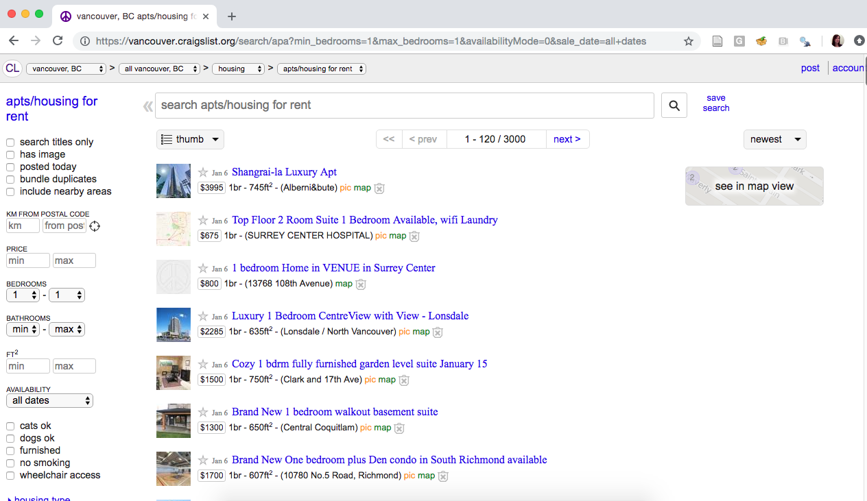
From that page, it’s pretty easy for our human eyes to find the apartment price and square footage. But how can we do this programmatically so we don’t have to copy and paste all these numbers? Well, we have to deal with the webpage source code, which we show a snippet of below (and link to the entire source code here):

        <span class="result-meta">
                <span class="result-price">$800</span>

                <span class="housing">
                    1br -
                </span>

                <span class="result-hood"> (13768 108th Avenue)</span>

                <span class="result-tags">
                    <span class="maptag" data-pid="6786042973">map</span>
                </span>

                <span class="banish icon icon-trash" role="button">
                    <span class="screen-reader-text">hide this posting</span>
                </span>

            <span class="unbanish icon icon-trash red" role="button" aria-hidden="true"></span>
            <a href="#" class="restore-link">
                <span class="restore-narrow-text">restore</span>
                <span class="restore-wide-text">restore this posting</span>
            </a>

        </span>
    </p>
</li>
         <li class="result-row" data-pid="6788463837">

        <a href="https://vancouver.craigslist.org/nvn/apa/d/north-vancouver-luxury-1-bedroom/6788463837.html" class="result-image gallery" data-ids="1:00U0U_lLWbuS4jBYN,1:00T0T_9JYt6togdOB,1:00r0r_hlMkwxKqoeq,1:00n0n_2U8StpqVRYX,1:00M0M_e93iEG4BRAu,1:00a0a_PaOxz3JIfI,1:00o0o_4VznEcB0NC5,1:00V0V_1xyllKkwa9A,1:00G0G_lufKMygCGj6,1:00202_lutoxKbVTcP,1:00R0R_cQFYHDzGrOK,1:00000_hTXSBn1SrQN,1:00r0r_2toXdps0bT1,1:01616_dbAnv07FaE7,1:00g0g_1yOIckt0O1h,1:00m0m_a9fAvCYmO9L,1:00C0C_8EO8Yl1ELUi,1:00I0I_iL6IqV8n5MB,1:00b0b_c5e1FbpbWUZ,1:01717_6lFcmuJ2glV">
                <span class="result-price">$2285</span>
        </a>

    <p class="result-info">
        <span class="icon icon-star" role="button">
            <span class="screen-reader-text">favorite this post</span>
        </span>

            <time class="result-date" datetime="2019-01-06 12:06" title="Sun 06 Jan 12:06:01 PM">Jan  6</time>


        <a href="https://vancouver.craigslist.org/nvn/apa/d/north-vancouver-luxury-1-bedroom/6788463837.html" data-id="6788463837" class="result-title hdrlnk">Luxury 1 Bedroom CentreView with View - Lonsdale</a>

This is not easy for our human eyeballs to read! However, it is easy for us to use programmatic tools to extract the data we need by specifying which HTML tags (things inside < and > in the code above). For example, if we look in the code above and search for lines with a price, we can also look at the tags that are near that price and see if there’s a common “word” we can use that is near the price but doesn’t exist on other lines that have information we are not interested in:

<span class="result-price">$800</span>

and

<span class="result-price">$2285</span>

What we can see is there is a special “word” here, “result-price”, which appears only on the lines with prices and not on the other lines (that have information we are not interested in). This special word and the context in which is is used (learned from the other words inside the HTML tag) can be combined to create something called a CSS selector. The CSS selector can then be used by R’s rvest package to select the information we want (here price) from the website source code.

Now, many websites are quite large and complex, and so then is their website source code. And as you saw above, it is not easy to read and pick out the special words we want with our human eyeballs. So to make this easier, we will use the SelectorGadget tool. It is an open source tool that simplifies generating and finding CSS selectors. We recommend you use the Chrome web browser to use this tool, and install the selector gadget tool from the Chrome Web Store. Here is a short video on how to install and use the SelectorGadget tool to get a CSS selector for use in web scraping:

From installing and using the selectorgadget as shown in the video above, we get the two CSS selectors .housing and .result-price that we can use to scrape information about the square footage and the rental price, respectively. The selector gadget returns them to us as a comma separated list (here .housing , .result-price), which is exactly the format we need to provide to R if we are using more than one CSS selector.

2.8.2 Are you allowed to scrape that website?

BEFORE scraping data from the web, you should always check whether or not you are ALLOWED to scrape it! There are two documents that are important for this: the robots.txt file and reading the website’s Terms of Service document. The website’s Terms of Service document is probably the more important of the two, and so you should look there first. What happens when we look at Craigslist’s Terms of Service document? Well we read this:

“You agree not to copy/collect CL content via robots, spiders, scripts, scrapers, crawlers, or any automated or manual equivalent (e.g., by hand).”

source: https://www.craigslist.org/about/terms.of.use

Want to learn more about the legalities of web scraping and crawling? Read this interesting blog post titled “Web Scraping and Crawling Are Perfectly Legal, Right?” by Benoit Bernard (this is optional, not required reading).

So what to do now? Well, we shouldn’t scrape Craigslist! Let’s instead scrape some data on the population of Canadian cities from Wikipedia (who’s Terms of Service document does not explicilty say do not scrape). In this video below we demonstrate using the selectorgadget tool to get CSS Selectors from Wikipedia’s Canada page to scrape a table that contains city names and their populations from the 2016 Canadian Census:

2.8.3 Using rvest

Now that we have our CSS selectors we can use rvest R package to scrape our desired data from the website. First we start by loading the rvest package:

library(rvest)

library(rvest) gives error…

If you get an error about R not being able to find the package (e.g., Error in library(rvest) : there is no package called ‘rvest’) this is likely because it was not installed. To install the rvest package, run the following command once inside R (and then delete that line of code): install.packages("rvest").

Next, we tell R what page we want to scrape by providing the webpage’s URL in quotations to the function read_html:

page <- read_html("https://en.wikipedia.org/wiki/Canada")

Then we send the page object to the html_nodes function. We also provide that function with the CSS selectors we obtained from the selectorgadget tool. These should be surrounded by quotations. The html_nodes function select nodes from the HTML document using CSS selectors. nodes are the HTML tag pairs as well as the content between the tags. For our CSS selector td:nth-child(5) and example node that would be selected would be: <td style="text-align:left;background:#f0f0f0;"><a href="/wiki/London,_Ontario" title="London, Ontario">London</a></td>

population_nodes <- html_nodes(page, "td:nth-child(5) , td:nth-child(7) , .infobox:nth-child(122) td:nth-child(1) , .infobox td:nth-child(3)")
head(population_nodes)

## {xml_nodeset (6)}
## [1] <td style="text-align:right;">5,928,040</td>
## [2] <td style="text-align:left;background:#f0f0f0;"><a href="/wiki/London,_Ontario" title="London, O ...
## [3] <td style="text-align:right;">494,069\n</td>
## [4] <td style="text-align:right;">4,098,927</td>
## [5] <td style="text-align:left;background:#f0f0f0;">\n<a href="/wiki/St._Catharines" title="St. Cath ...
## [6] <td style="text-align:right;">406,074\n</td>

Next we extract the meaningful data from the HTML nodes using the html_text function. For our example, this functions only required argument is the an html_nodes object, which we named rent_nodes. In the case of this example node: <td style="text-align:left;background:#f0f0f0;"><a href="/wiki/London,_Ontario" title="London, Ontario">London</a></td>, the html_text function would return London.

population_text <- html_text(population_nodes)
head(population_text)

## [1] "5,928,040"              "London"                 "494,069\n"              "4,098,927"             
## [5] "St. Catharines–Niagara" "406,074\n"

Are we done? Not quite… If you look at the data closely you see that the data is not in an optimal format for data analysis. Both the city names and population are encoded as characters in a single vector instead of being in a data frame with one character column for city and one numeric column for population (think of how you would organize the data in a spreadsheet). Additionally, the populations contain commas (not useful for programmatically dealing with numbers), and some even contain a line break character at the end (\n). Next chapter we will learn more about data wrangling using R so that we can easily clean up this data with a few lines of code.